Iowa Liquor Sales
October 12, 2016Jocelyn Ong
Where in Iowa should we open a liquor store?
Introduction
This is Project 3 from the Data Science Immersive at General Assembly and we’ll be working with the Iowa Liquor Sales dataset. This is also our first group project, and I’ll be collaborating with JP and Joshua.
For our project, we’ll be looking at the data from a market research perspective:
A liquor store owner in Iowa is looking to expand to new locations and has hired you to investigate the market data for potential new locations. The business owner is interested in the details of the best model you can fit to the data so that his team can evaluate potential locations for a new storefront.
About the dataset
How we obtained the data
The dataset we’ll be using can be downloaded directly from the data.iowa.gov website. It’s a large dataset and to facilitate working with the data, we’ll be looking at this dataset, which is 10% of a filtered version of the original dataset.
On a side note, the slightly filtered version can be found here version.
What’s in the data
According to data.iowa.gov:
This dataset contains the spirits purchase information of Iowa Class “E” liquor licensees by product and date of purchase…
Class E liquor license, for grocery stores, liquor stores, convenience stores, etc., allows commercial establishments to sell liquor for off-premises consumption in original unopened containers.
Here’s what the raw data looks like when we read it using Pandas:
| Column name | Data type | Description |
|---|---|---|
| Date | String | Date of liquor order |
| Store Number | Integer | Unique number assigned to each store |
| City | String | City where the store is located |
| Zip Code | String | Zip code where the store is located |
| County Number | Float | Iowa county number for the county where the store is located |
| County | String | County where the store is located |
| Category | Float | Category code associated with the liquor ordered |
| Category Name | String | Category of the liquor ordered |
| Vendor Number | Integer | The vendor number of the company for the brand of liquor ordered |
| Item Number | Integer | Item number for the individual liquor product ordered |
| Item Description | String | Description of the individual liquor product ordered |
| Bottle Volume (ml) | Integer | Volume of each liquor bottle in milliliters |
| State Bottle Cost | String | The amount that Alcoholic Beverages Division paid for each bottle of liquor ordered |
| State Bottle Retail | String | The amount the store paid for each bottle of liquor ordered |
| Bottles Sold | Integer | The number of bottles of liquor ordered by the store |
| Sale (Dollars) | String | Total cost of liquor order (number of bottles multiplied by the state bottle retail) |
| Volume Sold (Liters) | Float | Total volume of liquor ordered in liters (i.e. (Bottle Volume (ml) x Bottles Sold)/1,000) |
| Volume Sold (Gallons) | Float | Total volume of liquor ordered in gallons (i.e. (Bottle Volume (ml) x Bottles Sold)/3785.411784) |
What do we want to do
To recap, we want to use the data to help a liquor store owner decide where are the best locations for a new storefront.
Before we dove into the data wrangling, we wanted to clearly define what we would need for the above:
- Annual sales by location
- Annual volume (liter) by location
- Average cost per liter of liquor by location
- Number of stores in each location
Exploratory data analysis
We want our model to predict total sales and volume for each zip code. To do this, we would first need to compute total sales and total volume by zip code.
In our model, we want to exclude outlier stores, as these would represent stores that were doing exceptionally well or poorly - i.e. not your average store. We want to be able to tell an average store, if you open up another store in X zip code, you’ll have a better chance of doing well than if you open up in Y zip code.
To do this, we looked at the distribution of total sales by store.
# Aggregate sales and volume by stores
agg_columns = ['Sale (Dollars)', 'Volume Sold (Liters)']
store_summary = df2.groupby('Store Number')[agg_columns].sum().reset_index()
store_summary.columns = ['Store Number', 'Store Sales', 'Store Volume']
Plotting the above, this is the distribution we got:
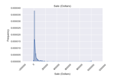
Because most of the stores had total annual sales of below $100,000, we set it as our threshold and dropped all stores that had total annual sales greater than $100,000. Doing so, we get the following distribution:
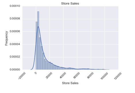
The distribution is still slightly skewed, but much less than before.
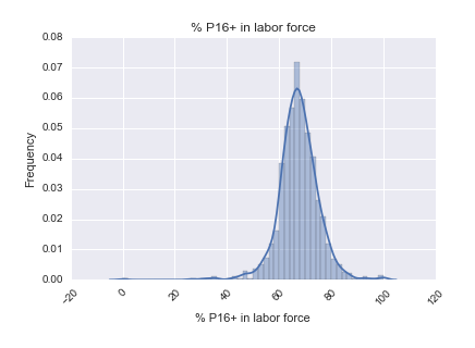
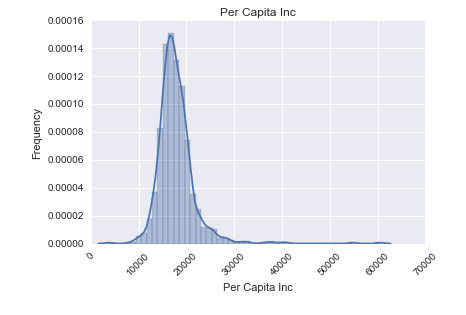
Looking at our original dataset, we felt that the available data was not sufficient for predicting sales per zip code. Our hypothesis is that the demographics of a zip code would have an influence on its liquor sales, so we found the demographic data for the zip codes in Iowa.
Here’s a look at the distributions of some of the columns in our demographic data:
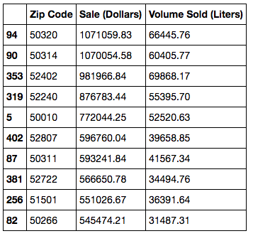
And here’s a quick look at which were the 10 best performing zips (without any cleaning/ removing of outliers).
Data munging/ data wrangling
We decided to look into zip codes as our location indicator.
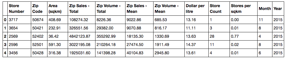
Using pivot tables, we generated the columns for total sales, total volume, and average price per liter for each zip code. We also generated store count by zip codes and store per square kilometer for our results table later on.
# Aggregate sales and volume by zip code
zip_summary = df3.groupby('Zip Code')[store_aggs].sum().reset_index().dropna()
zip_summary.columns = ['Zip Code', 'Zip Sales - Total', 'Zip Volume - Total']
df3 = df3.merge(zip_mean, how='left', on='Zip Code').drop_duplicates()
# Add store count
num_stores = df3[['Zip Code','Store Number']].drop_duplicates()
num_stores = num_stores.groupby('Zip Code').count().reset_index()
num_stores.columns = ['Zip Code', 'Store Count']
df3 = df3.merge(num_stores, how='left', on='Zip Code')
# Add a column for price per liter based on mean sales and mean volumes
df3['Dollar per liter'] = df3['Zip Sales - Total']/df3['Zip Volume - Total']
df3.head()
# Add stores per square kilometer
df3['Stores per sqkm'] = df3['Store Count']/df3['Area (sqkm)']
We then dropped the columns that we didn’t require (e.g. county, city, vendor number etc.).
Many of our columns in our demographic data were scaled differently so we used StandardScaler in sklearn.preprocessing to perform the scaling on the demographic data.
# scale the demo_data
demo_data_scaled = demo_data.copy()
cols_scale = demo_data_scaled.columns.values.tolist()[1:]
scaler = StandardScaler().fit(demo_data_scaled[cols_scale])
scaled_values = scaler.transform(demo_data_scaled[cols_scale])

for i in range(len(cols_scale)):
    demo_data_scaled[cols_scale[i]] = [x[i] for x in scaled_values]
All these data were then joined together to produce the final dataframe that we would be working with for building our model.
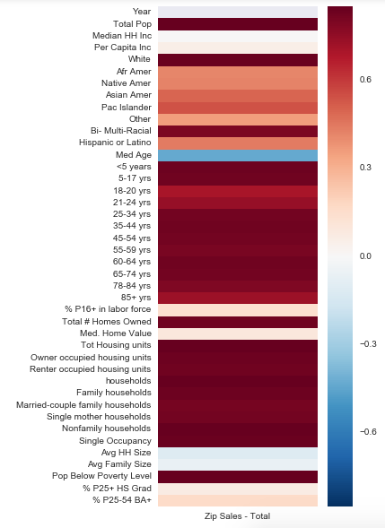
With these data, we first took a look at how our demographics were related to sales and volume:
Sales
Volume
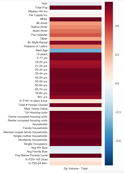
How to read the heatmaps: In this case, the colors of the heatmap range from dark blue to white to dark red. Where the colors are darker (red or blue) it indicates a stronger correlation (red for positive, blue for negative) between the feature and total sales/ volume. Where the colors are pale and closer to white, it indicates little or no correlation. Ideally, we would want to see more dark colors.
Modeling: generating the model and drawing conclusions
We built two models, one to predict sales, and one to predict volume. In both models, our features were the same - our demographic data.
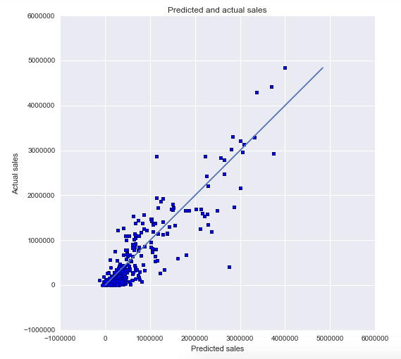
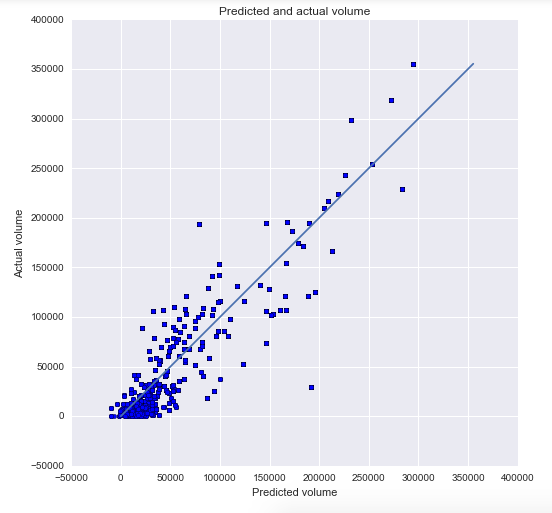
We chose lasso regression with cross validation to build our models and plotted our predicted values against our actual values to see how well the models did:
Sales - R-squared: 0.85
Volume - R-squared: 0.86
We then used our models to predict the expected sales and volume for all zip codes in Iowa (that we had demographic data for). With the total sales and total volume, we could then compute the average price per liter of alcohol.
predict_df['Predicted Total Sales'] = model_sales.predict(X_predict)
predict_df['Predicted Total Volume'] = model_volume.predict(X_predict) all_volume
predict_df['Predicted Dollar/liter'] = predict_df['Predicted Total Sales']/predict_df['Predicted Total Volume']
To decide where to open a new liquor store, a store owner would want to know which zip code has the best sales. On top of that, he’ll need to know what types of liquor are selling well: the cheaper ones or the more expensive ones? And how many other stores are there in that zip code right now: is it saturated?
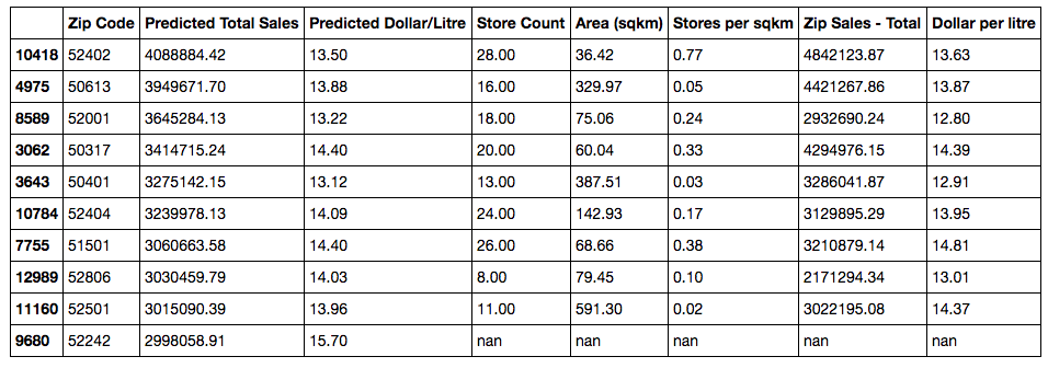
We sorted our zip codes firstly by total expected sales, then included the price per liter, total number of stores per zip code, and stores per square kilometer to address these questions.
Review: Challenges faced
We faced several problems with this project.
First, the dataset. We looked at the dataset and we couldn’t find anything that could help us predict where the best zip was. Thanks to JP and Joshua, we looked into demographics as a possible factor that affected liquor sales.
There were also lots of mistakes in the dataset: wrong zips, cities spelled wrongly, missing data etc. We managed to cut down the amount of cleaning required by using an external dataset for zip codes and other location data, even though it took quite a bit of work to collate these from the web (here and here).
Finally if you take a look at the data dictionary again, you’ll realize that there isn’t a field which talks about the profit or revenue of the liquor stores. The dollar values in our dataset refer to a) how much the state of Iowa paid to purchase the alcohol (presumably from distilleries/ breweries etc.); and b) how much the state of Iowa received from the liquor stores for the alcohol.
To deal with this, we made an assumption that a liquor store will be able to sell everything that it bought from the state within a short period of time (before the next transaction) and that the alcohol will never be sold at a loss.
The additional data that we brought in was also not ideal - we wanted to match the demographic data by year, but this information is not readily available for free (not yet at least). So we used what demographic data was available to us on the assumption that demographics for an area should not change drastically. I expect that with more detailed demographic data (year to year), we may get different results in our predictions. (Maybe not in the top 10 best locations, but probably in predicted sales and predicted price per liter of alcohol.)
Personal challenges
A challenge that I had personally that is not directly related to this project (but became really apparent during the course of the project) is writing neat code.
I have a tendency to throw code into the Jupyter notebook as and when ideas come into my head. As expected, the notebook usually turns out disorganized and it makes it difficult to read and follow the flow of ideas. Since I only noticed this when I finished most of the code for the project, I found it really difficult to go back and add comments to my code and move them around.
I ended up creating a new notebook with a planned flow, and copying code from the original notebook into the new notebook with proper comments and variable names. That took quite a while and it was a good reminder to me to do plan my code and comment it as I write it to avoid all these in future.
Until next time
We had a couple of ‘next steps’ that we came up with for our project which I plan to look into at a later date:
- What made the outlier stores outliers? (i.e. is there any particular reason they were spending so much more on buying alcohol from the state as compared to other stores?)
- What are possible pricing strategies once you’ve chosen a zip code?
- We noted that some of our predictions turned out negative (which doesn’t make sense for sales or volume)
- Possible solution: log transformation, what is log transformation, when do you use it and will it work in this case?
- Is there an optimal inventory that we can predict from this dataset?
In addition to the above, we were also provided with another scenario where we were the data scientist in residence at the Iowa State tax board and were supposed to look at the data with the objective of liquor sales projections for the future so as to determine liquor tax rates. This may be another project that I’ll look into on the side.
Thank you for reading and I hope you found the above interesting!
You can view my notebook for this project here.
Back to top ↑