Hierarchical Clustering In Scipy

Understanding the SciPy code behind hierarchical clustering

Hierarchical Clustering

Today we looked at hierarchical clustering, and while I understood the concept, I struggled with trying to understand how the code worked - what goes where and what preprocessing steps are required? Now that I’ve figured it out (sort of), I want to share what I learned with you!

The Concept

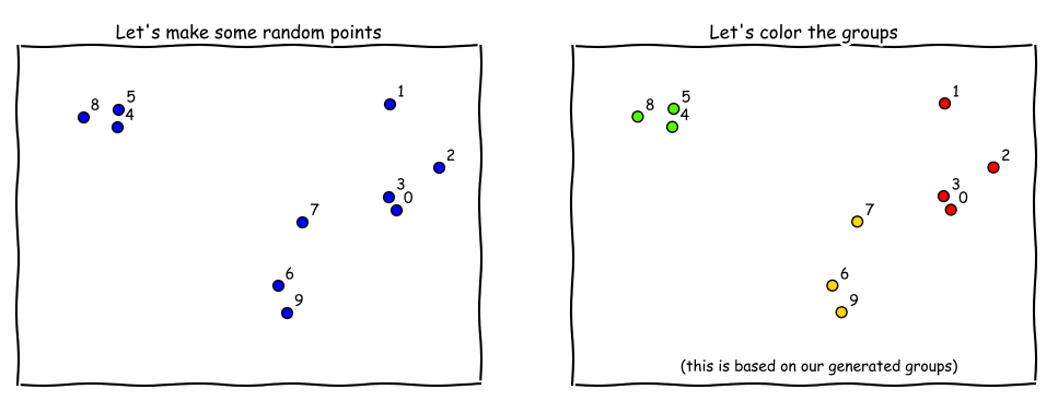
In clustering, our aim is to group some points. Any number of points, in any number of dimensions, into any number of groups. For ease of explanation, we’ll look at points in a 2-dimensional space.

Using datasets.make_blobs in sklearn, we generated some random points (and groups) - each of these points have two attributes/ features, so we can plot them on a 2D plot (see below).

X, y = make_blobs(n_samples=10,
                  cluster_std=2.5,
                  random_state=77)

With hierarchical clustering, we look at the “distance” between all the points, and we group them pairwise by smallest “distance” first. We will need to decide what is our distance measure first. At each step, we only group two points/ clusters. Once a cluster is formed, it is considered as one unit at the next step.

In our example, it looks like points 0 and 3 are the closest, so they’re grouped, and in the next step, we only consider the distances between [1, 2, 4, 5, 6, 7, 8, 9, 10, (0,3)] <- 9 units. Once we start to have clusters, that’s where our distance measure comes into play. Do we compare the nearest points to find the distance between two clusters, or the farthest, or maybe the average? (As we all know, the answer, as it is 99.9% of the time, is it depends.)

This order of grouping can be displayed in a dendrogram. (What’s a dendrogram?)

from scipy import cluster
Z = cluster.hierarchy.linkage(X, "complete")
cluster.hierarchy.dendrogram(Z);

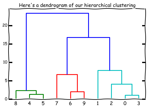
The height of each little “bracket” is representative of the distance between points/ clusters as well as the order the grouping is done (the shortest ones go first).

You’ll notice that the tree goes all the way up to the top - where all the points are in one big cluster. That’s usually not our objective - we usually want the points in n groups, where n < number of points. With hierarchical clustering, we can look at the dendrogram and decide how many clusters we want.

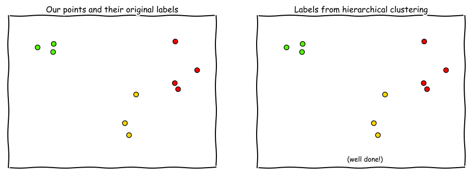
cut = cluster.hierarchy.fcluster(Z, 10, criterion="distance")

In clustering, we get back some form of labels, and we usually have nothing to compare them against. But in this case, we want to see how well the clustering did so we’d want to compare the labels and see if they match up. Unfortunately, even if the clusters are grouped correctly, the labels may not match up - a class 0 may be labeled as cluster 2, class 1 -> cluster 5 etc.

So we’ll try to map the cluster labels back to the original labels. (Note: this doesn’t always work, but we shouldn’t need to too often, perhaps only when we’re trying to test a clustering method.)

labs = np.zeros_like(cut)
for i in np.unique(cut):
    mask = (cut == i)
    labs[mask] = stats.mode(y[mask])[0]

With this, we can use classification metrics (e.g. accuracy, precision, recall, f1-score etc.) to see how well our clustering model did.

Or we can plot it so that the same colors are generated on each plot, and just look at it visually to determine how well we did.

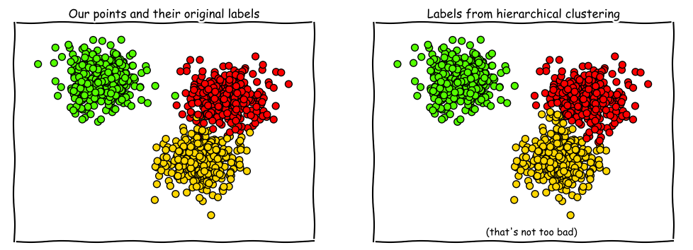
Here’s a comparison with more points.

Digging deeper into the code

That all seems nice and easy, right? (It wasn’t.)

What format does our data have to be in to be able to run cluster.hierarchy.linkage on it?

We read the documentation:

scipy.cluster.hierarchy.linkage(y, method=’single’, metric=’euclidean’)

Parameters:

y : ndarray
A condensed or redundant distance matrix. A condensed distance matrix is a flat array containing the upper triangular of the distance matrix. This is the form that pdist returns. Alternatively, a collection of mm observation vectors in n dimensions may be passed as an mm by nn array.

method : str, optional
The linkage algorithm to use. See the Linkage Methods section below for full descriptions.

metric : str or function, optional
The distance metric to use in the case that y is a collection of observation vectors; ignored otherwise. See the distance.pdist function for a list of valid distance metrics. A custom distance function can also be used. See the distance.pdist function for details.

Returns:

Z : ndarray
The hierarchical clustering encoded as a linkage matrix.

Okay, so y must be a matrix. What does condensed or redundant mean? What shape does y have to be? I still haven’t figured out what condensed or redundant means yet, but I’ve got a pretty good idea of what y needs to look like.

In the source code for clustering.hierarchy.linkage, the function checks the dimension of y. To put it simply, the dimension of an array is the number of levels there are within the array. If you have a flat array (i.e. no nested arrays), dimension = 1. If you have an array of arrays, dimension = 2. It you have an array of arrays of arrays, dimension = 3. And so on.

linkage only takes y with dimensions of 1 or 2. When dimension == 1, the elements in y are the distances between the points, and the length of y is (p choose 2) or (p * (p-1)) / 2 where p = number of points. Clustering then takes place using these distances.

But our data usually doesn’t come like that. What we usually get is a whole bunch of features for each point, where each feature represents one dimension.

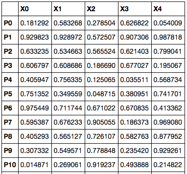
This can be represented as a 2-dimensional array (an array of arrays), which is acceptable as a y in clustering.hierarchy.linkage. In this case, there is an extra step, where distance between each P is calculated using scipy.spatial.distance.pdist. Clustering is then using the result of those calculated distances.

Or maybe, you’ll get a dataframe where both the index and columns are references to points, and each element is the distance between the index-point and the column-point. Something like this:

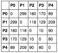
In this case, the grid is symmetrical along the diagonal and we’ll need to extract the figures from one of the triangles formed by this diagonal.

from scipy import spatial
y = spatial.distance.squareform(distance_grid)

This returns an array of the distances between the points which can then be passed into cluster.hierarchy.linkage!

Until next time

I really hope this post helped you understand the functions a little better. I didn’t go through all the functions or parameters, just the ones that tripped me up and took some staring at the source code to understand.

You can view my notebook here.

If you have any comments/ questions on this post or if you’d like to discuss further, feel free to tweet me or drop me an email!