Billboard Hot 100

What can we tell about the songs on the Billboard Hot 100?

What is the data about

As someone who doesn’t listen much to anything apart from ‘classical’ music, I didn’t even know what the Billboard Hot 100 was. And for the sake of people like me (if there are any others), I’ll just go through a little of what it is.

I had to read quite a few articles and links on the Billboard Hot 100 before I could figure out how the data worked. Here’s the gist of it:

From Wikipedia

The Billboard Hot 100 is the music industry standard record chart in the United States for singles, published weekly by Billboard magazine. Chart rankings are based on radio play, online streaming, and sales (physical and digital).

Also here

Ideally, any effective genre chart—be it R&B, Latin, country, even alt-rock—doesn’t just track a particular strain of music, which can be marked by ever-changing boundaries and ultimately impossible to define. It’s meant to track an audience.

Another from Wikipedia

What separates the charts is which stations and stores are used; each musical genre has a core audience or retail group. Each genre’s department at Billboard is headed up by a chart manager, who makes these determinations.

Essentially, the Billboard Hot 100 is a list of tracks that are ranked in the top 100 by radio play, online streaming and sales; the genre that the song is listed under is determined by its audience and not by its artist.

What’s in the data

The dataset includes the artist’s name, track name, track length, genre, the date it entered the Hot 100, the date it reached its highest rank on the Hot 100, and its rank on the Hot 100 for a period of 75 weeks starting from the week it entered (each week is represented as one column).

Problem Statement

This week in class, we learned about defining a problem statement or a hypothesis. In layman terms, a problem statement or a hypothesis is a statement which you want to prove is true (or disprove).

1. Does the rank at which a track enters the top 100 have any relation to whether it will eventually reach the top 10?
2. Does the length of a track have any relation to its highest rank attainable?

Exploratory data analysis (EDA)

Before we dive into the problem statement, we should take a look at the dataset and determine if any data cleaning is required.

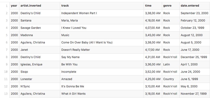
The original dataset has 317 entries of the tracks which were in the Hot 100 in the year 2000.

In the weeks where a track was no longer in the Hot 100, the value is passed as an asterisk (*). To facilitate our EDA, we’ll tell pandas to treat asterisks as null values.

df = pd.read_csv('assets/billboard.csv', na_values='*')

The ‘time’ column actually refers to the length of the track, and is currently formatted as ‘MM, SS, MS AM’ where MM refers to minutes, SS to seconds and MS to milliseconds (e.g. 3,38,00 AM - the AM appears as a result of formatting). We’ll format it to return the length of a track in seconds.

The ‘genre’ column has some typos and a couple of categories which only appear once or twice. We’ll clean up the spelling differences and group the minorities as ‘Others’. Here, we’ll define minorities as anything that appears less than 1% of the time. Doing so, we’re left with the genres ‘Rock’, ‘Country’, ‘Rap’, ‘R&B’, and ‘Others’.

From the ‘date.entered’ and ‘date.peaked’ columns, we can find out how many weeks each track took to reach its highest rank; from the columns of the 75 weeks tracked, we can find out the rank that a track entered the Hot 100, and the number of weeks a track stayed on the Hot 100.

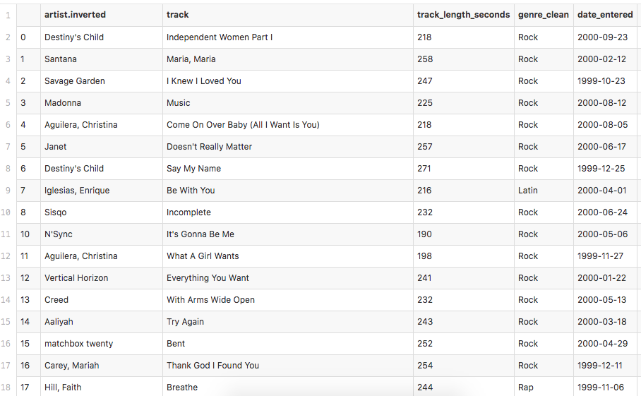
Here’s a snapshot of our cleaned dataset:

Statistics of our dataset

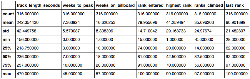
What we can tell from the above:

• ‘weeks_to_peak’ has a minimum value of 0
  • There are track(s) which hit their highest rank the moment they got into top 100
• ‘weeks_to_peak’ has a median value of 7
  • On average, it takes a track 7 weeks to hit its highest rank
• ‘weeks_on_billboard’ has a median value of 18
  • On average, tracks stayed in the top 100 for 18 weeks
• ‘weeks_on_billboard’ has a minimum value of 1
  • There are track(s) which were only in the top 100 for a week

Going back to what we wanted to find out

Does the rank at which a track enters the Hot 100 have any relation to whether or not it will eventually reach the top 10?

This problem statement seems to require just two subsets of data from the dataset: the highest rank obtained by each track and the rank which the track entered. Let’s plot these two sets of data to see if there are any immediately discernible patterns.

sns.pairplot(df,x_vars='rank_entered', y_vars='highest_rank', size=5);

We can see from the pairplot that no matter what the ranks were coming into the Hot 100, there were tracks which got to the top 10.

To test our problem statement, we should see if there is any difference between the average entering rank of tracks that hit the top 10 and tracks that do not. We will use median as our measure of average so that the result is not too highly skewed by outliers.

To be a little more specific, our null hypothesis is that top 10 tracks have the same median rank entering the Hot 100 as non-top 10 tracks.

df2['rank_entered'][df2['reached_top_10'] == False].median() - df2['rank_entered'][df2['reached_top_10'] == True].median()

The above returns a value of about 8.

Our dataset shows that the average entering rank of tracks which become top 10 hits is at least 8 ranks above those which do not make the top 10. However, since our dataset is small, this may not be a conclusive finding.

In the absence of a bigger dataset for the same year (i.e. 2000), we’ll use a permutation test to find the probability of getting a difference of 8 or more ranks between top 10 tracks and non-top 10 tracks.

In this permutation test, we are treating the data as if the rank at which a track enters the Hot 100 has no relation to whether it gets into the top 10 eventually.

To do this, we randomize the data for the ranks entering the Hot 100, and assign each rank to either the group which reaches the top 10 or the group which doesn’t. The proportion of the groups should be the same as the original dataset.

We’ll set our significance level at 5%: if the probability of getting a difference of at least 8 is less than 5%, then there is a relationship between the rank a track entered the Hot 100 and whether it reaches a top 10 position.

trials = 100000
counter = 0
t1 = df2['rank_entered']
top_L = df2['track'][df2['reached_top_10'] == True].count()
for i in range(trials):
    t2 = np.random.permutation(t1)
    top = t2[:top_L]
    bottom = t2[top_L:]
    diff = np.median(bottom) - np.median(top)
    if diff >= 8:
        counter += 1.0000
print 'p-value: {}%'.format((counter/trials)*100)

Running the above a couple of times, the probability that we get back is very small, much smaller than 5%. Hence, we can reject the hypothesis that there is no relationship between rank entered and whether a track will reach the top 10 (i.e. the two are related - if Track A comes into the Hot 100 at a higher rank than Track B, there is a higher chance of A being in the top 10 than B).

However, it is not immediately clear how the two are related (whether one can be predicted from the other, or how closely they are related). More data may be required to determine this.

Does the length of a track have any relation to its highest rank attainable?

This problem statement is actually similar to the one above. In this instance, our null hypothesis is that the length of a track has no relation to its highest rank.

Let’s first take a look at the distribution of the data:

To test this, we grouped our data into two groups - long tracks and short tracks. How youwould define whether a track was long or short is purely arbitrary - we defined a long track as one that is longer than 250 seconds for a good distribution between the two groups.

We found that the median highest rank of the short tracks was 9 ranks better than the median highest rank of the long tracks. Again, due to the small sample size, we used the permutation test to find out the probability of getting this result if we assumed that the null hypothesis is true (i.e. length of a track had no relation to its highest rank).

We returned a very high probability of that (almost 14%) - i.e. we do not reject the null hypothesis. It seems like track length and highest rank are not related!

Looking at other possible factors that affect the highest rank

Let’s take a look at the data using Tableau!

Using Tableau, we can add in additional dimensions to our plot. In the above, we’ve included the season which a track entered the Hot 100 and the number of weeks it spent on the Hot 100.

Just looking at it visually, we can see that there aren’t many tracks which were on the Hot 100 for a short period of time that were in the top 10 (the smaller circles tend to be more to the right of the chart).

It’s not as obvious for seasons, but it does seem like there’s more yellow and blue on the left side of the chart (tracks which enter the Hot 100 in Spring and Fall are more likely to have made it to the top 10).

Again, we can’t tell much about the data, except that there might be some correlation.

Until next time

This week, we looked at how to clean data to get it ready for analysis and how to test a problem statement using permutation testing.

I hope you enjoyed this post, and I look forward to bringing you more insights on data science.

You can view my notebook for this project here.