Disaster Survival Classification
October 25, 2016Jocelyn Ong
Can we predict who will survive a disaster?
Introduction
This week we’re looking at a classification problem, and we’ll consider various classification models and how they compare to one another. In this week’s scenario:
You’re working as a data scientist with a research firm that specializes in emergency management. In advance of client work, you’ve been asked to create and train a logistic regression model that can show off the firm’s capabilities in disaster analysis.
How would this be useful to an emergency management firm? Maybe it can be used to predict the probability of survival in a disaster for efficient resource allocation (very contentious discussion here - we’ll not go into that), or maybe it can be used as an after-the-fact review, to see if there were any factors that affected the survival rate.
About the dataset
We’ll be working with the very well-used Titanic dataset. We were told to pull the data from the General Assembly database using SQL, but if you’d like to work with the dataset on your own, it is also available on Kaggle.
We pulled the data using the iPython-sql magic and psycopg. You can view the documentation and installation instructions here and here.
Data dictionary
| Column | Type | Description |
|---|---|---|
| PassengerID | Integer | Numerical identifier for each passenger |
| Survived | Binary (Integer) | Whether the passenger survived (0 = No; 1 = Yes) |
| Pclass | Categorical (Integer) | Passenger Class (1 = 1st; 2 = 2nd; 3 = 3rd); Pclass is a proxy for socio-economic status (1st ~ Upper; 2nd ~ Middle; 3rd ~ Lower) |
| Name | String | Passenger name |
| Sex | Binary (String) | Sex (male; female) |
| Age | Float | Passenger age in years Fractional if age less than one, xx.5 if estimated |
| SibSp | Integer | Number of siblings/ spouses aboard (Brother, sister, stepbrother, or stepsister; husband or wife) |
| Parch | Integer | Number of parents/ children aboard (Mother or father, son, daughter, stepson or stepdaughter) |
| Ticket | String | Ticket Number |
| Fare | Float | Amount paid for ticket |
| Cabin | String | Cabin number |
| Embarked | Categorical (String) | Port of embarkation (C = Cherbourg; Q = Queenstown; S = Southampton) |
The above information is obtained from Kaggle and formatted for presentation purposes.
The column “Survived” is our target, and the rest of the columns may be used as features (where data is complete and relevant).
Exploratory Data Analysis (EDA)
For our EDA, we’ll look at the various columns in relation to the column “Survived” and see if we can find any relationships just from visualizations.
Plots:
-
Class and sex

-
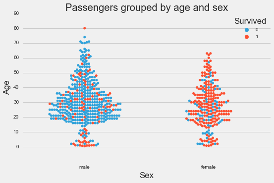
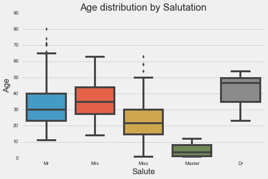
Age and sex
-
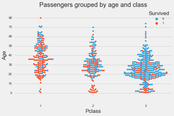
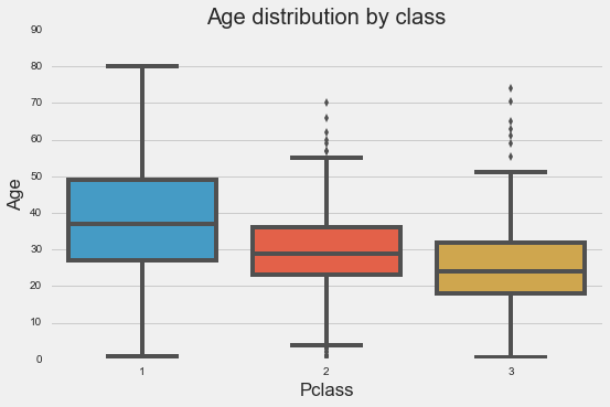
Age and class
-
Age and port of embarkation

Based on the plots, we can see that age, sex and class seem to be good indications of whether a passenger survived or not. Port of embarkation seems to have some indication, but because majority of the passengers boarded at Southampton, we can’t tell for sure whether there’s any effect.
We can also take a look at the heatmap of the correlations in our dataset:
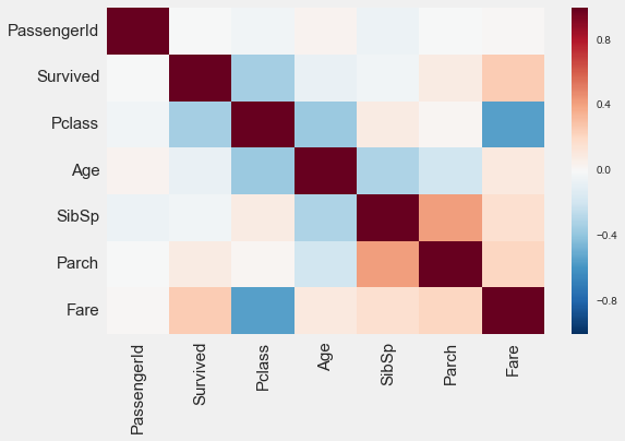
The heatmap tells us the strength of the correlation between “Survived” and each of the other columns, and also tells us if there is any multicollinearity between the other columns.
(So what if there is? Multicollinearity in our features may affect interpretability of our model, so if we would like to be able to say what affects our predictions, we may want to avoid any multicollinearity issues.)
Based on our EDA, it seems like age, class, and sex might be good predictors in our model. Port of embarkation may be a good predictor but it seems like most of the passengers got on at Southampton, so we’re not sure if this will have a big impact.
Data wrangling
Now that we’ve identified some of the features that we may want to use in our model, we’ll need to examine each of these columns to see if any preprocessing is required.
Missing values
Let’s look at our dataset to identify any missing values:
df.info()
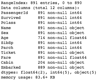
Age was supposed to be one of our main features, but there are so many missing instances! We don’t have a lot of data, so let’s try to fill these in.
(It would have been interesting to look at cabins and location of the cabins and see how this might have affected whether a passenger would survive or not, but there are too many of these missing and no obvious way for us to impute the values, so we’ll leave cabin out for now.)
One way we could fill in the missing values in age is to just fill in the median age in all the blanks. But maybe we can go one step further. Let’s see what we can use to find age:
-
Class
-
Salutation
-
Class and salutation
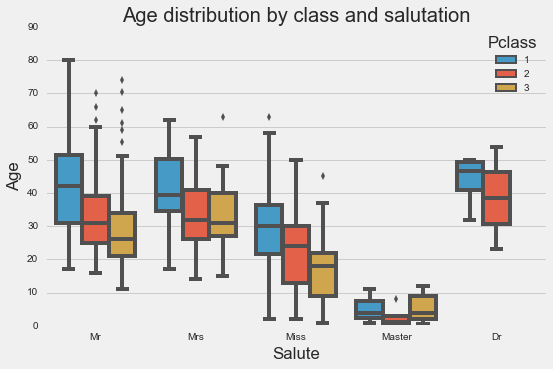
It seems like if we combine class and salutation, we may be able to get a more accurate estimation of age.
Backtrack a few steps: how do we get a passenger’s salutation?
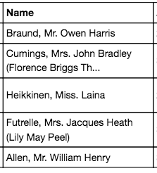
Each “Name” entry is in the format Last Name, Salutation. First Name. The salutations all have a period to it, so we’ll split the names on spaces, and look for the item that has a period, and return that.
def get_salute(name):
    name_list = name.split(',')
    name_list = name_list[1].strip().split(' ')
    salute = [i for i in name_list if '.' in i]
    return salute[0].strip('.')
There were a few salutations which only occurred a few times, so we grouped them into the majority groups, and ended up with the five main salutations. We then found the median age of each salutation and class.
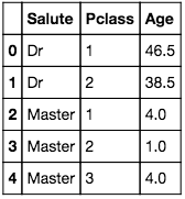
Each missing age in our dataset is then mapped to this to return an estimated age.
Dummy variables
In our next preprocessing step, we’ll create dummy variables for our categorical data using pd.get_dummies.
df = pd.get_dummies(df, columns=["Sex", "Pclass", "Embarked"], drop_first=True)
This creates dummy columns for “Sex”, “Pclass”, “Embarked”, and drops the original columns in the dataframe as well as one of the dummy columns for each item.
Using dummies for categorical data removes any ‘order’ implied in using numerical categories.
Scaling continuous variables
Next, we’ll scale our continuous variables so that they are comparable. We will use StandardScaler in sklearn.preprocessing for this.
Before we perform the scaling, we’ll split our data into train and test sets, so that we can test our model with data that it has not encountered before.
# Split the X and y into training and test sets
X_train, X_test, y_train, y_test = train_test_split(df2[all_features],df2['Survived'],stratify=df2['Survived'], test_size=0.33, random_state=77)

# Create a StandardScaler instance
scaler = StandardScaler()

# fit the scaler to the train data
scaler = scaler.fit(X_train[scale_features])
# For each column we want to scale, create a new column with the prefix Scaled_ for the training data
for i in range(len(scale_features)):
    X_train['Scaled_'+scale_features[i]] = [x[i] for x in scaler.transform(X_train[scale_features])]
# Now do the same for X_test
for i in range(len(scale_features)):
    X_test['Scaled_'+scale_features[i]] = [x[i] for x in scaler.transform(X_test[scale_features])]
Note that we’ve only trained our scaler on the training data, and that our test data is scaled on the same scale as the training data.
Modeling: generating the model and drawing conclusions
We’ll be looking at four different classification models - logistic regression, K nearest neighbors, decision tree, and bagging classifier.
We’ll also run gridsearch on each of these classifiers to get the best parameters for each.
Logistic regression
gs = GridSearchCV(LogisticRegression(),
                 logreg_parameters,
                 cv=5)
gs.fit(X_train,y_train)
K Nearest neighbors
gs2 = GridSearchCV(KNeighborsClassifier(),
                   {'n_neighbors': np.arange(1,50,5),
                    'weights': ['uniform', 'distance'],
                    'algorithm': ['ball_tree', 'kd_tree', 'brute']},
                   cv=5)
gs2.fit(X_train,y_train)
Decision tree classifier
gs4 = GridSearchCV(DecisionTreeClassifier(),
                   {'criterion': ['gini', 'entropy'],
                    'min_samples_split': np.arange(2,30,2),
                    'min_samples_leaf': np.arange(1,15,1)},
                   cv=5)
gs4.fit(X_train, y_train)
Bagging classifier
gs5 = GridSearchCV(BaggingClassifier(base_estimator=dt),
                  {'n_estimators': np.arange(10,50,5),
                  'max_samples': np.arange(0.1,1.0,0.1),
                  'max_features': np.arange(1,len(X_train.columns)+1,1)},
                  cv=5)
gs5.fit(X_train, y_train)
With our four models, we plotted our ROC curves on the same plot to compare them:
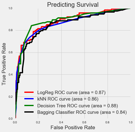
All four curves are actually very similar and it’s difficult to tell which of these is considered the best. If you wanted to be really particular, you would first decide what your tradeoff would be between your true positive rate (TPR) and false positive rate (FPR). This would give you a line (vertical or horizontal depending on whether you wanted to limit TPR or FPR) which would intersect all four curves, and you’d pick the one that had the best performance at that point. (Otherwise, the performance of any of the curves should be comparable in general.)
Feature importance
So how important were the features we used in determining whether a passenger survived?
There are a few ways we can interpret this, and we’ll consider two of them now.
Logistic regression coefficients
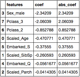
We’ve ranked the features in order of the magnitude of their absolute coefficients. This number is an indication of how much the feature affects the model.
We can see that at the top of our table is whether the passenger is male (or not). Which kind of makes sense if you think about the movie - “Women and children first!”.
Class comes next. Specifically, whether a passenger was in the third class or not. If we go back up to our EDA, you’ll see that most of the third class passengers did not survive, so it seemed logical that the model would place more importance on this.
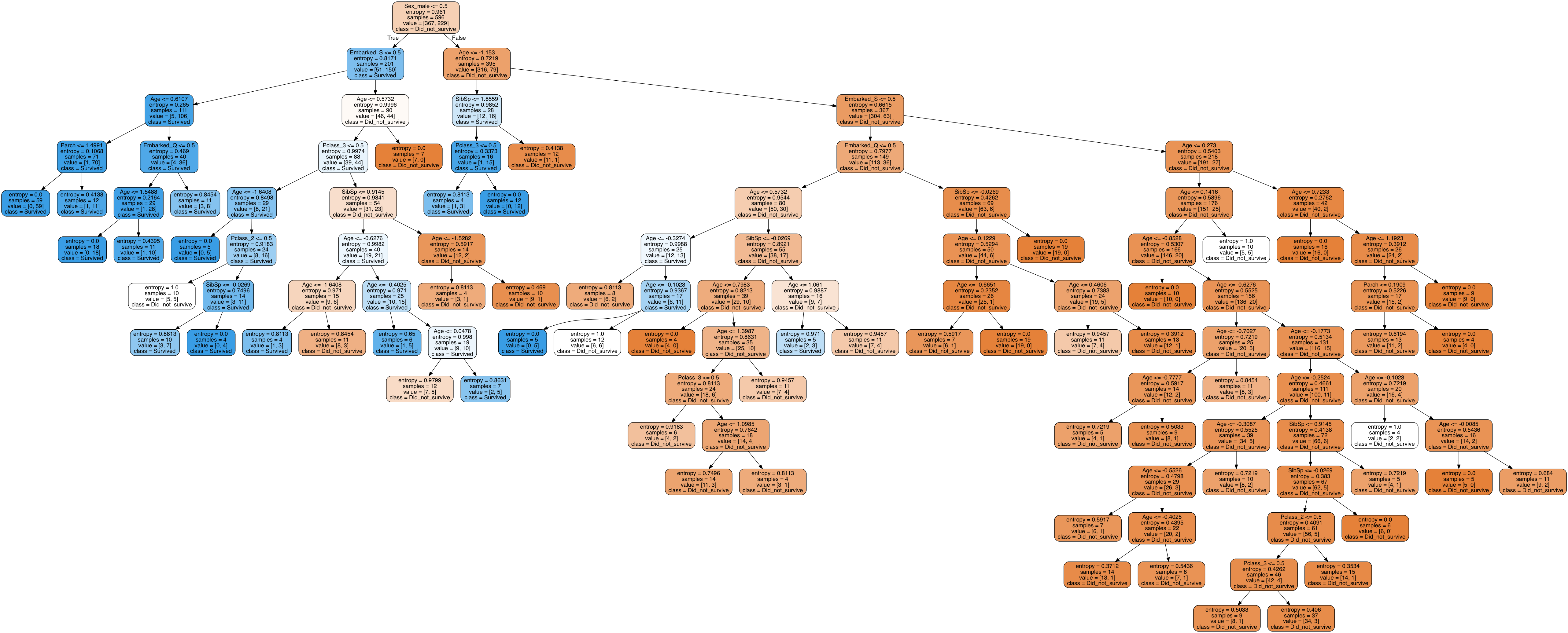
Decision tree
Another way to interpret feature importances is to look at how our decision tree was constructed. The goal of a decision tree is to reach purity in the least number of steps. Another way to look at it, is that at each step, the decision tree asks a question that separates the data most clearly into each class.
We’ve exported our decision tree into an image file and it’s massive (many decision trees are), but right at the top is again whether the the passenger is male (or not).
Round up
This is a well studied dataset and you can definitely find many posts online exploring it. Despite that, I hope you’ve enjoyed reading about my exploration of the Titanic dataset! I enjoyed working with it and it was also a good chance to work on my visualization skills.
You can view my notebook for this project here.
Stay tuned for my next post!
Back to top ↑